pAPRika tutorial 2 - Explicit Solvent
In this example, we will setup and simulate butane (BUT) as a guest molecule for the host cucurbit[6]uril (CB6).
Unlike the previous tutorial, in this one, we will solvate the host-guest complex in water with additional Na+ and Cl- ions. This tutorial builds off tutorial 1. I’ve marked new pieces of information with a blue circle, like so:
🔵 Since we have a prepared host-guest-dummy setup from the first tutorial, I’m going to skip the initial tleap steps and go right into initializing the restraints.
🔵 The default mode of pAPRika is to detect whether a simulation has completed successfully, and if so, skip that window. This helps when launching mulitple jobs on a cluster or queuing system that might kill jobs after a pre-determined time. That means that running this notebook with the same set of windows as the first tutorial will not re-run the simulations and the results won’t change. The easiest thing to do is to rename or delete the existing windows directory, if you would like to
compare the results between the two methods.
Initial Setup
[ ]:
import os
data = "../../../paprika/data/cb6-but"
Determine the number of windows
Before we add the restraints, it is helpful to set the \(\lambda\) fractions that control the strength of the force constants during attach and release, and to define the distances for the pulling phase.
The attach fractions go from 0 to 1 and we place more points at the bottom of the range to sample the curvature of \(dU/d \lambda\). Next, we generally apply a distance restraint until the guest is ~18 Angstroms away from the host, in increments of 0.4 Angstroms. This distance should be at least twice the Lennard-Jones cutoff in the system. These values have worked well for us, but this is one aspect that should be carefully checked for new systems.
[1]:
attach_string = "0.00 0.40 0.80 1.60 2.40 4.00 5.50 8.65 11.80 18.10 24.40 37.00 49.60 74.80 100.00"
attach_fractions = [float(i) / 100 for i in attach_string.split()]
[2]:
import numpy as np
initial_distance = 6.0
pull_distances = np.arange(0.0 + initial_distance, 18.0 + initial_distance, 1.0)
These values will be used to measure distance relative to the first dummy atom, hence the addition of 6.00.
[3]:
release_fractions = []
[4]:
windows = [len(attach_fractions), len(pull_distances), len(release_fractions)]
print(f"There are {windows} windows in this attach-pull-release calculation.")
There are [15, 18, 0] windows in this attach-pull-release calculation.
Alternatively, we could specify the number of windows for each phase and the force constants and targets will be linearly interpolated. Other ways of specifying these values are documented in the code.
Add restraints using pAPRika
pAPRika supports four different types of restraints:
Static restraints: these six restraints keep the host and in the proper orientation during the simulation (necessary),
Guest restraints: these restraints pull the guest away from the host along the \(z\)-axis (necessary),
Conformational restraints: these restraints alter the conformational sampling of the host molecule (optional), and
Wall restraints: these restraints help define the bound state of the guest (optional).
More information on these restraints can be found in:
Henriksen, N.M., Fenley, A.T., and Gilson, M.K. (2015). Computational Calorimetry: High-Precision Calculation of Host-Guest Binding Thermodynamics. J. Chem. Theory Comput. 11, 4377–4394. DOI
In this example, I will show how to setup the static restraints and the guest restraints.
We have already added the dummy atoms and we have already defined the guest anchor atoms. Now we need to define the host anchor atoms (H1, H2, and H3) in the above diagram. The host anchors should be heavy atoms distributed around the cavity (and around the pulling axis). One caveat is that the host anchors should be rigid relative to each other, so conformational restraints do not shift the alignment of the pulling axis relative to the solvation box. For CB6, I have chosen carbons around the central ridge.
[5]:
G1 = ":BUT@C"
G2 = ":BUT@C3"
[6]:
H1 = ":CB6@C"
H2 = ":CB6@C31"
H3 = ":CB6@C18"
I’ll also make a shorthand for the dummy atoms.
[7]:
D1 = ":DM1"
D2 = ":DM2"
D3 = ":DM3"
Static restraints
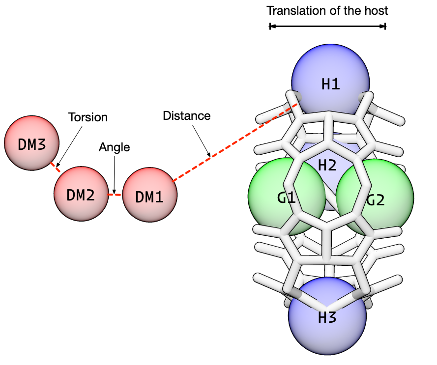
These harmonic restraints are constant throughout the entire simulation. These restraints are used to control the distances and angles between the host and guest relative to the dummy atom. We have created a special class for these restrains, static_DAT_restraint, that uses the initial value as the restraint target (this is why the starting structure should be a reasonable facsimile of the bound state).
Note that these restraints are not “attached” and they don’t need to be “released” – their force constants do not change in magnitude.
The first three static restraints affect the translational distance, angle, and torsion angle between the host and the dummy atoms. These control the position of the host, via the first anchor atom, from moving relative to the dummy atoms.
There is no correct value for the force constants. From experience, we know that a distance force constant of 5.0 kcal/mol/\(\overset{\circ}{\text{A}}\)\(^2\) won’t nail down the host and yet it also won’t wander away. Likewise, we have had good results using 100.0 kcal/mol/\(rad^2\) for the angle force constant.
[8]:
from paprika import restraints
static_restraints = []
[9]:
import parmed as pmd
structure = pmd.load_file("complex/cb6-but-dum.prmtop", "complex/cb6-but-dum.rst7")
[10]:
r = restraints.static_DAT_restraint(restraint_mask_list = [D1, H1],
                                    num_window_list = windows,
                                    ref_structure = structure,
                                    force_constant = 5.0,
                                    amber_index=True)

static_restraints.append(r)
[11]:
r = restraints.static_DAT_restraint(restraint_mask_list = [D2, D1, H1],
                                    num_window_list = windows,
                                    ref_structure = structure,
                                    force_constant = 100.0,
                                    amber_index=True)

static_restraints.append(r)
[12]:
r = restraints.static_DAT_restraint(restraint_mask_list = [D3, D2, D1, H1],
                                    num_window_list = windows,
                                    ref_structure = structure,
                                    force_constant = 100.0,
                                    amber_index=True)

static_restraints.append(r)
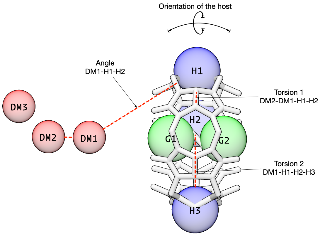
The next three restraints control the orientation of the host relative to the dummy atoms. These angle and torsion restraints prevent the host from rotating relative to the dummy atoms.
[13]:
r = restraints.static_DAT_restraint(restraint_mask_list = [D1, H1, H2],
                                    num_window_list = windows,
                                    ref_structure = structure,
                                    force_constant = 100.0,
                                    amber_index=True)

static_restraints.append(r)
[14]:
r = restraints.static_DAT_restraint(restraint_mask_list = [D2, D1, H1, H2],
                                    num_window_list = windows,
                                    ref_structure = structure,
                                    force_constant = 100.0,
                                    amber_index=True)

static_restraints.append(r)
[15]:
r = restraints.static_DAT_restraint(restraint_mask_list = [D1, H1, H2, H3],
                                    num_window_list = windows,
                                    ref_structure = structure,
                                    force_constant = 100.0,
                                    amber_index=True)

static_restraints.append(r)
Guest restraints
Next, we add restraints on the guest. These restraints control the position of the guest and are the key to the attach-pull-release method. During the attach phase, the force constants for these restraints is increased from zero. During the pull phase, the target for the distance restraint is increased (in the orange box, below), translating the guest away from the host cavity. And during the release phase, the force constants are reduced from their “full” value back down to zero.
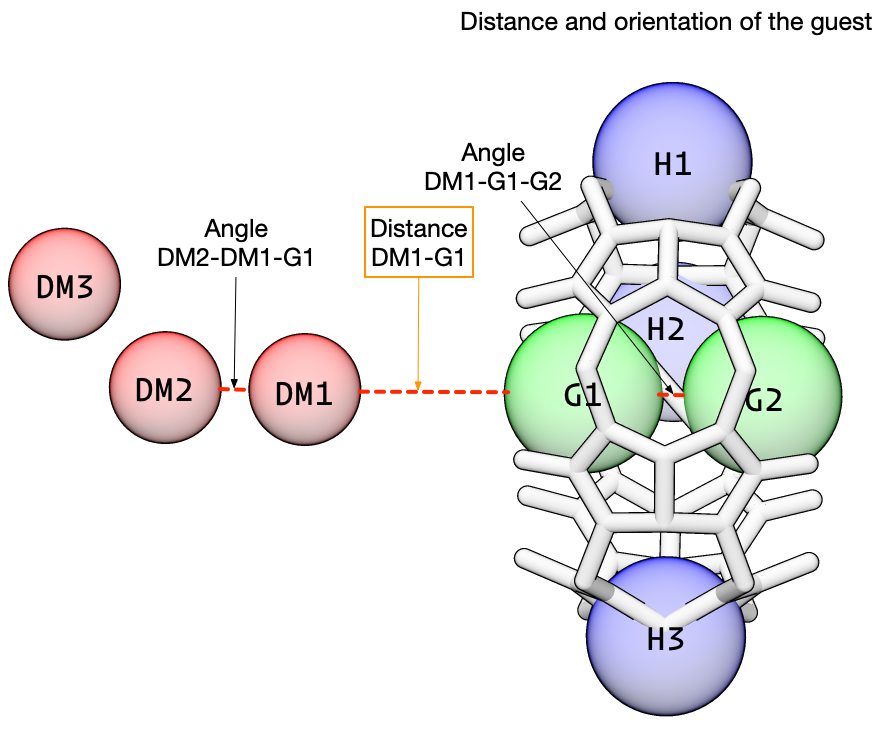
We use the class DAT_restraint to create these three restraints. We will use the same anchor atoms as before, with the same distance and angle force constants. Note that unlike static_DAT_restraint, we will first create the restraint, then set the attributes, then initialize the restraint which does some checks to make sure everything is copacetic.
There are two additional convenience options here:
auto_apr = Truesets the force constant during pull to be the final force constant after attach and sets the initial restraint target during pull to be the final attach target.continuous_apr = Truesets the last window of attach to be the same as the first window as pull (and likewise for release)
Also note, due to a quirk with AMBER, we specifcy angle and torsion targets in degrees but the force constant using radians!
[16]:
guest_restraints = []
[17]:
r = restraints.DAT_restraint()
r.mask1 = D1
r.mask2 = G1
r.topology = structure
r.auto_apr = True
r.continuous_apr = True
r.amber_index = True

r.attach["target"] = 6.0                            # Angstroms
r.attach["fraction_list"] = attach_fractions
r.attach["fc_final"] = 5.0                          # kcal/mol/Angstroms**2

r.pull["target_final"] = 24.0                       # Angstroms
r.pull["num_windows"] = windows[1]

r.initialize()
guest_restraints.append(r)
[18]:
r = restraints.DAT_restraint()
r.mask1 = D2
r.mask2 = D1
r.mask3 = G1
r.topology = structure
r.auto_apr = True
r.continuous_apr = True
r.amber_index = True

r.attach["target"] = 180.0                          # Degrees
r.attach["fraction_list"] = attach_fractions
r.attach["fc_final"] = 100.0                        # kcal/mol/radian**2

r.pull["target_final"] = 180.0                      # Degrees
r.pull["num_windows"] = windows[1]

r.initialize()
guest_restraints.append(r)
[19]:
r = restraints.DAT_restraint()
r.mask1 = D1
r.mask2 = G1
r.mask3 = G2
r.topology = structure
r.auto_apr = True
r.continuous_apr = True
r.amber_index = True

r.attach["target"] = 180.0                          # Degrees
r.attach["fraction_list"] = attach_fractions
r.attach["fc_final"] = 100.0                        # kcal/mol/radian**2

r.pull["target_final"] = 180.0                      # Degrees
r.pull["num_windows"] = windows[1]

r.initialize()
guest_restraints.append(r)
Create the directory structure
We use the guest restraints to create a list of windows with the appropriate names and then we create the directories.
[20]:
import os
from paprika.restraints.restraints import create_window_list

window_list = create_window_list(guest_restraints)
for window in window_list:
    os.makedirs(f"windows/{window}")
Next, we ask pAPRika to write the restraint information in each window
In each window, we create a file named disang.rest to hold all of the restraint information that is required to run the simulation with AMBER. We feed the list of restraints to pAPRika, one by one, and it returns the appropriate line.
The functional form of the restraints is specified in section 25.1 of the AMBER18 manual. Specifically, these restraints have a square bottom with parabolic sides out to a specific distance and then linear sides beyond that. The square bottom can be eliminated by setting r2=r3 and the linear extension can be eliminated by setting the the r4 = 999 and r1 = 0, creating a harmonic restraint
[21]:
from paprika.restraints.amber import amber_restraint_line

host_guest_restraints = (static_restraints + guest_restraints)
for window in window_list:
    with open(f"windows/{window}/disang.rest", "w") as file:
        for restraint in host_guest_restraints:
            string = amber_restraint_line(restraint, window)
            if string is not None:
                file.write(string)
It is a good idea to open up the disang.rest files and see that the force constants and targets make sense (and there are no NaN values). Do the force constants for the guest restraints start at zero? Do the targets for the pull slowly increase?
Save restraints to a JSON file
🔵 The previous code block writes restraints in a format that AMBER uses to run simulations in each window, but pAPRika uses other information stored in the DAT_restraint class in the analysis module. By saving the restraints in a file, it is easy to chunk up setup, simulation, and analysis in different sessions orpython scripts.
Note: the API for saving and loading restraints is not stable and may be moved into another submodule. The output notes that pAPRika is not including the entire topology in the restraint JSON, but will contain a reference to the file that was used to setup th restraints, in this case, cb6-but-dum.prmtop.
[22]:
from paprika.io import save_restraints
[23]:
save_restraints(host_guest_restraints, filepath="windows/restraints.json")
Prepare host-guest system
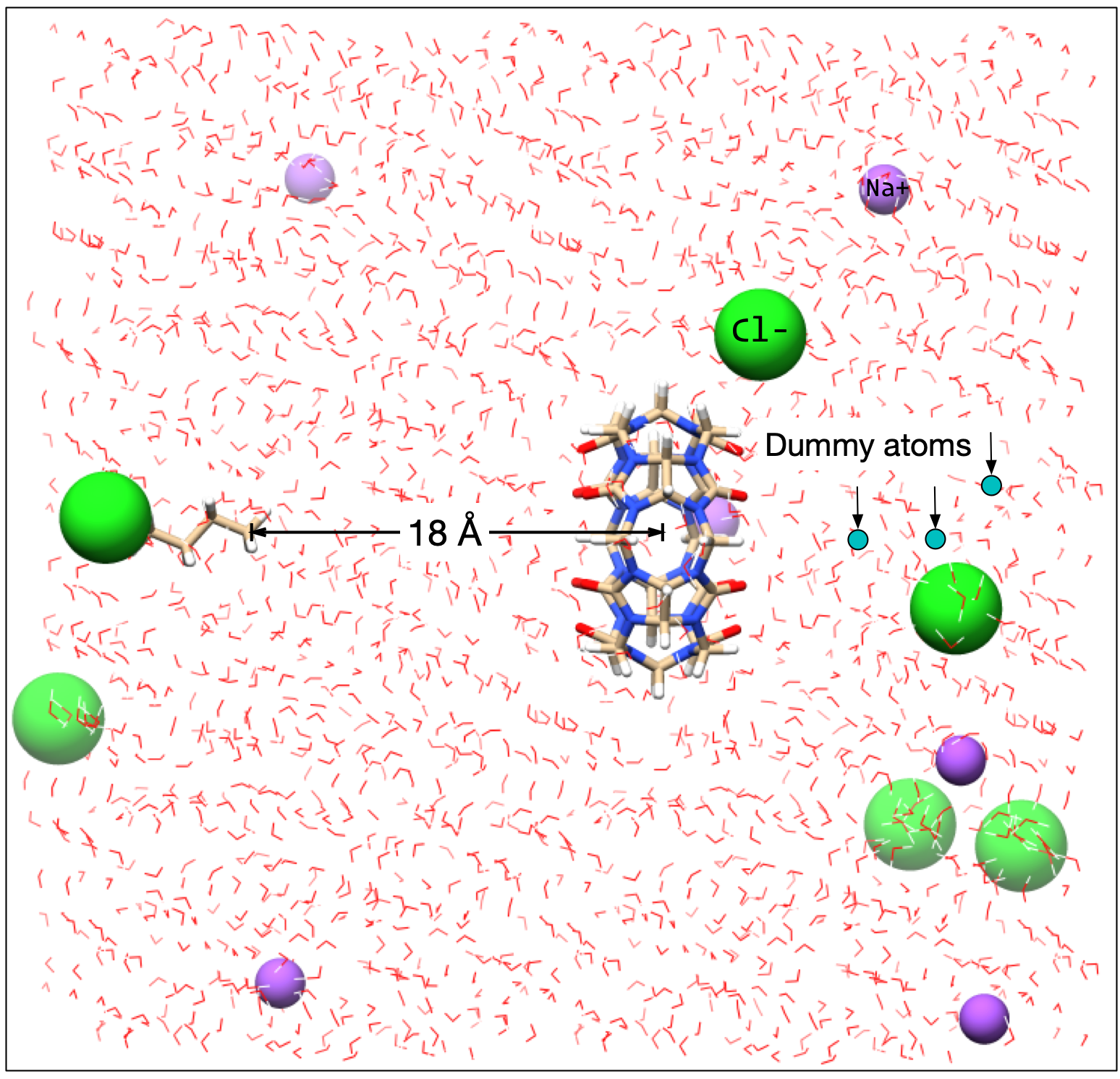
Translation of the guest (before solvation)
For the attach windows, we will use the initial, bound coordinates for the host-guest complex. Only the force constants change during this phase, so a single set of coordinates is sufficient. For the pull windows, we will translate the guest to the target value of the restraint before solvation, and for the release windows, we will use the coordinates from the final pull window.
[24]:
import shutil

for window in window_list:
    if window[0] == "a":
        shutil.copy("complex/cb6-but-dum.prmtop", f"windows/{window}/cb6-but-dum.prmtop")
        shutil.copy("complex/cb6-but-dum.rst7", f"windows/{window}/cb6-but-dum.rst7")
    elif window[0] == "p":
        structure = pmd.load_file("complex/cb6-but-dum.prmtop", "complex/cb6-but-dum.rst7",
                          structure = True)
        target_difference = guest_restraints[0].phase['pull']['targets'][int(window[1:])] - guest_restraints[0].pull['target_initial']
        print(f"In window {window} we will translate the guest {target_difference.magnitude:0.1f}.")
        for atom in structure.atoms:
            if atom.residue.name == "BUT":
                atom.xz += target_difference.magnitude
        structure.save(f"windows/{window}/cb6-but-dum.prmtop")
        structure.save(f"windows/{window}/cb6-but-dum.rst7")
In window p000 we will translate the guest 0.0 Angstroms.
In window p001 we will translate the guest 1.1 Angstroms.
In window p002 we will translate the guest 2.1 Angstroms.
In window p003 we will translate the guest 3.2 Angstroms.
In window p004 we will translate the guest 4.2 Angstroms.
In window p005 we will translate the guest 5.3 Angstroms.
In window p006 we will translate the guest 6.4 Angstroms.
In window p007 we will translate the guest 7.4 Angstroms.
In window p008 we will translate the guest 8.5 Angstroms.
In window p009 we will translate the guest 9.5 Angstroms.
In window p010 we will translate the guest 10.6 Angstroms.
In window p011 we will translate the guest 11.6 Angstroms.
In window p012 we will translate the guest 12.7 Angstroms.
In window p013 we will translate the guest 13.8 Angstroms.
In window p014 we will translate the guest 14.8 Angstroms.
In window p015 we will translate the guest 15.9 Angstroms.
In window p016 we will translate the guest 16.9 Angstroms.
In window p017 we will translate the guest 18.0 Angstroms.
Before running a simulation, open each window and check that the position of the host and dummy atoms are fixed and that the position of the guest is bound during the attach windows, moves progressively further during pull, and is away from the host during the release windows.
Solvate each window
🔵 Unlike the previous tutorial we will solvate the system in each window.
[25]:
from paprika.build.system import TLeap
By default, this will use cubic periodic boundary conditions; we usually use octahedral periodic boundary conditions to optimize space. Based on experience, 2000 waters is a resaonable amount for CB6, but sometimes it is necessary to run with 2500 or 3000 waters depending on the size of the host and guest molecules. The code below first neutralizes the system (which does not do anything here) and then adds an additional 6 Na+ and 6 Cl- ions. The counterion species can be changed via
counter_cation and counter_anion, and the add_ions string can take concentrations in the form of 0.150M or 0.150m for Molarity or molality, respectively.
Note that when running simulations with periodic boundary conditions, be mindful of the box size relative to the Lennard-Jones cutoff.
[26]:
for window in window_list:
    print(f"Solvating system in window {window}.")
    structure = pmd.load_file(f"windows/{window}/cb6-but-dum.prmtop",
                              f"windows/{window}/cb6-but-dum.rst7")

    if not os.path.exists(f"windows/{window}/cb6-but-dum.pdb"):
        structure.save(f"windows/{window}/cb6-but-dum.pdb")

    system = TLeap()
    system.output_path = os.path.join("windows", window)
    system.output_prefix = "cb6-but-dum-sol"

    system.target_waters = 2000
    system.neutralize = True
    system.add_ions = ["Na+", 6, "Cl-", 6]
    system.template_lines = [
        "source leaprc.gaff",
        "source leaprc.water.tip3p",
        f"loadamberparams {data}/cb6.frcmod",
        "loadamberparams ../../complex/dummy.frcmod",
        f"CB6 = loadmol2 {data}/cb6.mol2",
        f"BUT = loadmol2 {data}/but.mol2",
        "DM1 = loadmol2 ../../complex/dm1.mol2",
        "DM2 = loadmol2 ../../complex/dm2.mol2",
        "DM3 = loadmol2 ../../complex/dm3.mol2",
        "model = loadpdb cb6-but-dum.pdb",
    ]
    system.build()
Solvating system in window a000.
Solvating system in window a001.
Solvating system in window a002.
Solvating system in window a003.
Solvating system in window a004.
Solvating system in window a005.
Solvating system in window a006.
Solvating system in window a007.
Solvating system in window a008.
Solvating system in window a009.
Solvating system in window a010.
Solvating system in window a011.
Solvating system in window a012.
Solvating system in window a013.
Solvating system in window p000.
Solvating system in window p001.
Solvating system in window p002.
Solvating system in window p003.
Solvating system in window p004.
Solvating system in window p005.
Solvating system in window p006.
Solvating system in window p007.
Solvating system in window p008.
Solvating system in window p009.
Solvating system in window p010.
Solvating system in window p011.
Solvating system in window p012.
Solvating system in window p013.
Solvating system in window p014.
Solvating system in window p015.
Solvating system in window p016.
Solvating system in window p017.
Simulation
🔵 This is going to look very similar to the the implicit solvent simulation setup, except instead of using config_gb_min and config_gb_sim, we will use config_pdb_min and config_pbc_sim.
For this part, you need to have the AMBER executables in your path.
[27]:
from paprika.simulate import AMBER
Run a quick minimization in every window. Note that we need to specify simulation.cntrl["ntr"] = 1 to enable the positional restraints on the dummy atoms.
I’m using the logging module to keep track of time.
[28]:
import logging
from importlib import reload
reload(logging)

logger = logging.getLogger()
logging.basicConfig(
    format='%(asctime)s %(message)s',
    datefmt='%Y-%m-%d %I:%M:%S %p',
    level=logging.INFO
)
Energy Minimization
[29]:
for window in window_list:
    simulation = AMBER()
    simulation.executable = "mpirun -np 4 pmemd.MPI"

    simulation.path = f"windows/{window}/"
    simulation.prefix = "minimize"

    simulation.topology = "cb6-but-dum-sol.prmtop"
    simulation.coordinates = "cb6-but-dum-sol.rst7"
    simulation.ref = "cb6-but-dum-sol.rst7"
    simulation.restraint_file = "disang.rest"

    simulation.config_pbc_min()
    simulation.cntrl["ntr"] = 1
    simulation.cntrl["restraint_wt"] = 50.0
    simulation.cntrl["restraintmask"] = "'@DUM'"

    logging.info(f"Running minimization in window {window}...")
    simulation.run()
2020-10-05 12:18:34 PM Running minimization in window a000...
2020-10-05 12:19:00 PM Running minimization in window a001...
2020-10-05 12:19:26 PM Running minimization in window a002...
2020-10-05 12:19:52 PM Running minimization in window a003...
2020-10-05 12:20:18 PM Running minimization in window a004...
2020-10-05 12:20:45 PM Running minimization in window a005...
2020-10-05 12:21:11 PM Running minimization in window a006...
2020-10-05 12:21:37 PM Running minimization in window a007...
2020-10-05 12:22:03 PM Running minimization in window a008...
2020-10-05 12:22:29 PM Running minimization in window a009...
2020-10-05 12:22:56 PM Running minimization in window a010...
2020-10-05 12:23:22 PM Running minimization in window a011...
2020-10-05 12:23:48 PM Running minimization in window a012...
2020-10-05 12:24:14 PM Running minimization in window a013...
2020-10-05 12:24:40 PM Running minimization in window p000...
2020-10-05 12:25:07 PM Running minimization in window p001...
2020-10-05 12:25:33 PM Running minimization in window p002...
2020-10-05 12:25:59 PM Running minimization in window p003...
2020-10-05 12:26:25 PM Running minimization in window p004...
2020-10-05 12:26:51 PM Running minimization in window p005...
2020-10-05 12:27:17 PM Running minimization in window p006...
2020-10-05 12:27:44 PM Running minimization in window p007...
2020-10-05 12:28:10 PM Running minimization in window p008...
2020-10-05 12:28:36 PM Running minimization in window p009...
2020-10-05 12:29:02 PM Running minimization in window p010...
2020-10-05 12:29:28 PM Running minimization in window p011...
2020-10-05 12:29:54 PM Running minimization in window p012...
2020-10-05 12:30:20 PM Running minimization in window p013...
2020-10-05 12:30:47 PM Running minimization in window p014...
2020-10-05 12:31:13 PM Running minimization in window p015...
2020-10-05 12:31:39 PM Running minimization in window p016...
2020-10-05 12:32:05 PM Running minimization in window p017...
For simplicity, I am going to skip equilibration and go straight to production!
🔵 I’m also going to run a little bit longer in each window, because the additional atoms increases the convergence time. The total simulation time per window, in nanoseconds, is (nstlim) × (dt in fs / 1000) = (50000) × (0.002 / 1000) = 0.1 ns. This is still very short and just for demonstration. A production simulation might require as much as 15 ns per window for binding free energies and up to 1 us per window for binding enthalpies.
Production Run
[33]:
for window in window_list:
    simulation = AMBER()
    simulation.executable = "pmemd.cuda"
    simulation.gpu_devices = 0

    simulation.path = f"windows/{window}/"
    simulation.prefix = "production"

    simulation.topology = "cb6-but-dum-sol.prmtop"
    simulation.coordinates = "minimize.rst7"
    simulation.ref = "cb6-but-dum-sol.rst7"
    simulation.restraint_file = "disang.rest"

    simulation.config_pbc_md()
    simulation.cntrl["ntr"] = 1
    simulation.cntrl["restraint_wt"] = 50.0
    simulation.cntrl["restraintmask"] = "'@DUM'"
    simulation.cntrl["nstlim"] = 50000

    logging.info(f"Running production in window {window}...")
    simulation.run(overwrite=True)
2020-10-05 12:42:12 PM Running production in window a000...
2020-10-05 12:42:25 PM Running production in window a001...
2020-10-05 12:42:38 PM Running production in window a002...
2020-10-05 12:42:51 PM Running production in window a003...
2020-10-05 12:43:04 PM Running production in window a004...
2020-10-05 12:43:18 PM Running production in window a005...
2020-10-05 12:43:31 PM Running production in window a006...
2020-10-05 12:43:44 PM Running production in window a007...
2020-10-05 12:43:57 PM Running production in window a008...
2020-10-05 12:44:11 PM Running production in window a009...
2020-10-05 12:44:24 PM Running production in window a010...
2020-10-05 12:44:37 PM Running production in window a011...
2020-10-05 12:44:50 PM Running production in window a012...
2020-10-05 12:45:04 PM Running production in window a013...
2020-10-05 12:45:17 PM Running production in window p000...
2020-10-05 12:45:30 PM Running production in window p001...
2020-10-05 12:45:43 PM Running production in window p002...
2020-10-05 12:45:57 PM Running production in window p003...
2020-10-05 12:46:10 PM Running production in window p004...
2020-10-05 12:46:23 PM Running production in window p005...
2020-10-05 12:46:36 PM Running production in window p006...
2020-10-05 12:46:50 PM Running production in window p007...
2020-10-05 12:47:03 PM Running production in window p008...
2020-10-05 12:47:16 PM Running production in window p009...
2020-10-05 12:47:29 PM Running production in window p010...
2020-10-05 12:47:43 PM Running production in window p011...
2020-10-05 12:47:56 PM Running production in window p012...
2020-10-05 12:48:09 PM Running production in window p013...
2020-10-05 12:48:22 PM Running production in window p014...
2020-10-05 12:48:35 PM Running production in window p015...
2020-10-05 12:48:49 PM Running production in window p016...
2020-10-05 12:49:02 PM Running production in window p017...
Analysis
🔵 We will perform the analysis using restraints saved previously to a JSON file.
Once the simulation is completed, we can using the analysis module to determine the binding free energy. We supply the location of the parameter information, a string or list for the file names (wildcards supported), the location of the windows, and the restraints on the guest.
In this example, we use the method ti-block which determines the free energy using thermodynamic iintegration and then estimates the standard error of the mean at each data point using blocking analysis. Bootstrapping it used to determine the uncertainty of the full thermodynamic integral for each phase.
After running compute_free_energy(), a dictionary called results will be populated, that contains the free energy and SEM for each phase of the simulation.
[34]:
from paprika.io import load_restraints
[35]:
guest_restraints = load_restraints("windows/restraints.json")
[36]:
from paprika import analysis
[37]:
free_energy = analysis.fe_calc()
free_energy.topology = "cb6-but-dum-sol.prmtop"
free_energy.trajectory = 'production*.nc'
free_energy.path = "windows"
free_energy.restraint_list = guest_restraints
free_energy.collect_data()
free_energy.methods = ['ti-block']
free_energy.ti_matrix = "full"
free_energy.boot_cycles = 1000
free_energy.compute_free_energy()
[38]:
free_energy.compute_ref_state_work([
    guest_restraints[0], guest_restraints[1], None,
    None, guest_restraints[2], None
])
[39]:
binding_affinity = -1 * (
free_energy.results["attach"]["ti-block"]["fe"] + \
free_energy.results["pull"]["ti-block"]["fe"] + \
free_energy.results["ref_state_work"]
)

sem = np.sqrt(
free_energy.results["attach"]["ti-block"]["sem"]**2 + \
free_energy.results["pull"]["ti-block"]["sem"]**2
)
[42]:
print(f"The binding affinity for butane and cucurbit[6]uril = {binding_affinity:0.2f} +/- {sem:0.2f} kcal/mol")
The binding affinity for butane and cucurbit[6]uril = -11.62 +/- 1.47 kcal/mol
In the first tutorial, using implicit solvation, the binding affinity estimate was -9.00 +/- 5.53 kcal/mol. Now, the affinity estimate is more favorable, by almost 2 kcal/mol, and we’ve halved the uncertainty. As before, with more windows and more simulation time per window, this value would continue to be refined.
The experimental value is \(-RT \ln (280*10^3 M)\) = -7.44 kcal/mol.